Backpropagation Demystified
Backpropagation is a well-established approach to train a neural network. The main goal of training a neural network is to determine the optimum values of connection weights (parameters) of the neural network. Following equation is used to update the connection weights
where, $w_i$ is the connection weight and $\alpha$ is the learning rate. Learning rate $\alpha$ controls magnitude of the change in the connection weight on each step of training process.
In the above equation, the partial derivative of the $E(w_i)$ w.r.t $w_i$ gives the direction in which the weight should be modified to reduce the error. In the equation, the only computationally expensive operation is to compute partial derivative. Without using backpropagation approach, with the increase in the number of layers of neural network computional complexity of the partial derivative increase exponentially. Using backprogation technique, the partial derivative of error w.r.t connection weight can be computed efficienly.
Refresher: Intuitive meaning of derivative and partial derivative
Let’s assume is time allocated by a person for the exercise and is the weight of the person. The derivative of w.r.t. means if the person makes a small change in the time allocated for the exercise how much the weight will change. Mathematically, the derivative of w.r.t. is represented as .
We know that diet () also has an effect on the weight of the person. Analysis of change in the weight of the person w.r.t. a small change in the time allocated for the exercise keeping diet same is given by the partial derivative of w.r.t. . Mathematically, the partial derivative of w.r.t. is represented as . Similarly, if the person keeps the exercise time the same and makes a small change in the diet it is represented as the partial derivative of w.r.t. which is represented as .
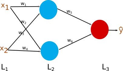
Figure 1: Toy neural network
Figure 1 shows the simplest possible neural network which is good enough to understand details of the backpropagation algorithm. In the figure, input-layer is layer-1 (), hidden-layer is () and output-layer is (). and are input to the neural network, blue nodes are nodes of hidden-layer and the red node is output-node. There are 6 connection weights to . In the training process we want to determine values of the connection weights which minimize error. In this post regression error is minimized to explain the backpropagation technique but the idea remains the same for the classification problem as well.
Square Error (E) =
As constant does not affect optimization problem, square of error is divided by 2 just to make the computation clean.
In Figure 1, each node (red/blue) represents three computations namely, multiplication of an input and a weight, sum of all the results of multiplications and finally activation score which is non-linearity of the summation. Figure 2 shows the clear and detailed view of the neural network which consists of multiplier, summation unit and non-linearity unit. Combination of the multiplier, summation and non-linearity function in Figure 2 is equivalent to a node in Figure 1.
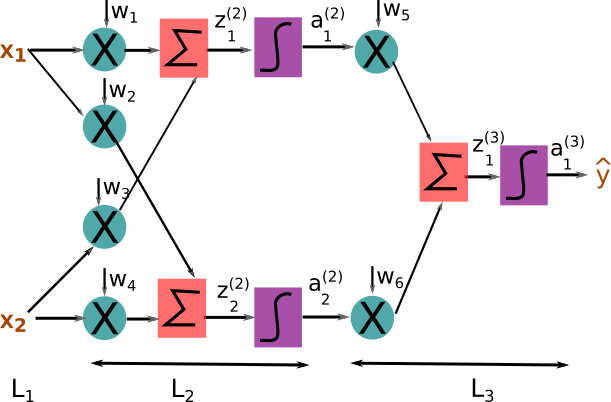
Figure 2: Equivalent detailed view of the toy neural network
is z of node-1 in layer-2 (Note: subscript => item number and superscript => layer-number) and is the activation score of node-1 in layer-2. Following equation is used to compute and in the figure 2
where, f() is a non-linearity function. Usually, non-linear function f() are sigmoid, tanh or Relu.
Backpropagation is all about computing partital derivative efficiently. Using backpropagation, we can calculate effectively where i = {1, 2, 3, 4, 5, 6}.
The partial derivative of error with respect to weight gives amount by which error will change if there is a small change in the weight. To calcualate the partial derivative of error w.r.t. weight chain rule is used.
To come up with the expression from Figure 1 can be confusing. However, if we construct a detailed view of the neural network as in Figure 2 then getting the expression is simply following chain rule from output to input (note it is backward). For to , the partial derivatives of error with respect to the weights can be calculated in the same way.
OMG!! expression of such a simple neural network is so complex. There will be total six partial derivatives, so how can we compute them effectively? The answer is dynamic programming. Dynamic programming is the fancy name of ** memorization and reutilization of computation.** We use the chain rule to get the expression of the partial derivative of error w.r.t. weights. To compute such complex expressions efficiently dynamic programming is used.
Layer-3
For ease of representation we represent as . Note that and have same sub-script (item-number) and superscript (layer-number).
To evaluate , the computation of can be utilized (memorized and reutilized) hence the repeated computation is avoided.
First chain rule is used to obtain the expression and then computaiton of is utilzed to compute . Following the similar steps, can be computed.
### Layer-2 The computations of layer-3 is reused for the computation of layer 2. Note that, computation starts from output toward input using the chain rule. The reutilization of the computation can be seen as message passing in the backward direction.
Similarly,
It is observed that term which appears in the computation of will be memorized and reutilized in the computation of .
Let’s calculate the partial derivative of error with respect to weight.
let’s say and Then,
We start with following expression, which looks like there is a lot of computation. But, utilizing the dynamic programming in each layer computation is minimized. Now, which looks much simpler and also computationally very efficient.
Similarly, the expression for the partial derivative of error w.r.t. remaining weights can be computed. We observed that if we break down a neural network into a detailed diagram as in Figure 2 then it would be easier to come up with chain rule. Once we have the expression, the long and complex expression can be computed efficiently using dynamic programming.